
Examining the Crab Nebula
In sixteen words, the task at hand was to determine some of the fundamental characteristics of the Crab Nebula. Observations were made several weeks ago from the 30 inch reflecting telescope at Leuschner Observatory
The Crab Nebula is the remnant of a star that went nova on July 4, 1054 as recorded by earthling observers. The nebula the the bulk of the star's mass that was ejected during the explosion and has been expanding ever since. The Nebula is a mass of hydrogen and helium roughly 2 parsecs(about 3x10^13 km) in diameter and is powered by the remnant of the star's core, the Crab pulsar at its core. The pulsar can be seen easily in the optical image, the first below.
In order to determine the rotation to the degree of precision required for the exercise, I wrote a procedure in IDL that found the centroid of each star to three decimal places. The idea for the image alignment I asked about in class, using a series of triangles to determine the offsets, scaling factors, and rotations of each image would have worked, however I chose in the interests of time to use the least squares fit method instead. The triangle method is probably at least as precise as the LSF, albeit more complex in execution. I also chose to follow the sage advice given in the writeup and stick to a linear LSF, solving for S Cos theta and S Sin theta (theta being the angle of rotation in radians) without the offsets built into the Fit process.
![]()
|
Image |
Rotation |
Scale Factor |
Variance in derived coefficients |
Wavelength (nm) |
|
Ultraviolet |
+.176 |
1.695 |
0.0015 |
110 |
|
Optical |
0 |
1.000 |
n/a |
550 |
|
Infra Red |
-.411 |
1.0059 |
0.013 |
1600 |
The above table has in its first column the angle through which the images had to rotated to be aligned with the Optical image. The second column, Scale Factor is the amount by which the images had to be expanded or compressed to match the scale of the Optical image. The Variance column is the variance is the parameters for the least squares fit of the alignment. As mentioned above, I did a linear fit with the parameters Ssin(�) and Scos(�), So the Variance column contains the variance in those derived quantities. The final column lists the wavelengths of each filter used to take each image.
The Crab Pulsar (smaller star of the central pair.)
Here is the Ultraviolet image of the Crab nebula, from the image taken by the mysterious 'B1' filter, shown in the blue/linear color table.
Above is a plot of the variances for the UV image and the IR image. The top line represents the UV variences and the bottom the IR. Where the minima occur is where the scale factor fits the images to one another best. The process that generated these curves was very suspect, as we seemed to have too much control over the shape of the graph. Because when whe took the variance over the whole image the graph closely resembeled an exponential curve with no clear minimum, we tried various box sizes in an attempt to get a coherant result. These curves used a 200 square pixel section and 150 square pixel section respectivly. The minima are appearantly near .92 for the UV and 1.02 for the IR. I cannot really say that the answers above are of any concequence because of the erratic behavior based of box sizes. I truly believe that given enough time, I could have found nearly any value for the minimum by choosing the correct box size and location of the image.
Near the edge of the nebula are regions of expanding gas that are moving faster than the general outer boundary of the nebula. These regions show up as tendrils poking through the nebula's surface. When I took the difference of two of the images, most of the features were canceled out, and the filaments became blured and non-descript. This would imply that the two fronts represented by the IR size and the UV size are fairly close to that of the optical image. My derived scale factors confirmed this, but our varience curves, upon closer inspection, yielded a troubling result. The optical image had a scale factor varience minimum smaller than one which would imply that it was larger than our IR image. I know this to not be the case, so there must have been some mishap in the calculations. The size of the nebula, if our finding were to have been in accordance with those of previous papers on the subject, should be proportional to the wavelength of the image taken to the 0.11 power. However, the predicted value of the size/wavelength ratio for the UV image to the optical was 1.19. What I actually found was a value of about 0.9 which implies that the UV image was larger than the optical image which is the opposite of what was to be expected..
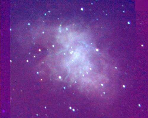
Below is a false color image of the nebula, composite from all three images. I transformed each of the images' intensities into a scale ranging from 0 to 255. The IR image is the red cnannel, the optical image is the green chanel, and the UV image is the blue channel.
![]() Pacific Standard Time
Pacific Standard Time
![]()
Hadrian is responsible for this one....
Special thanks to Kevin Burnett of http://www.xylem.demon.co.uk/kepler/altaz.html, a fine page indeed.